Boolean network attractors Landscape
Toy model
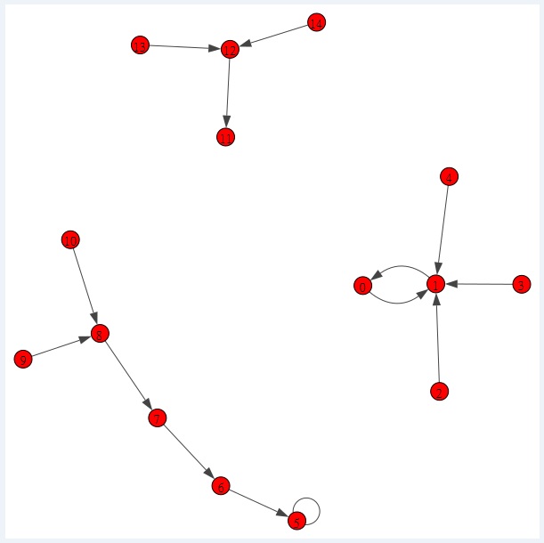
Below, we provide a toy model state transition graph. We use this toy model to demonstrate the intuitive method [1] for drawing the 3D landscape of Boolean network. This method is adapted from our Monte Carlo method for plotting Waddington's epigenetic landscape [2]. Here we explain an example how to estimate the probability distribution from trajectories in the state transition graph. Let us look at the trajectories to node 0. The trajectories to node 0 are: [1, 0] 1-->0; [2, 1, 0] 2-->1-->0; [3, 1, 0] 3-->1-->0; [4, 1, 0] 4-->1-->0 and [0]. We use a list named countn of length 15 (for 15 nodes) in Python for the counting of the trajectory passes each node. For example the trajectory [1, 0], add 1 to node 0 with index 0. For the trajectory [2, 1, 0], add 1 to node 1 and 0. Likewise we calculate for all the trajectories to each node. Then, for the estimate of the probability we divide each node count with the total. For details please read our paper [1].
 There are 15 nodes in the Boolean network. Node 5 and node 11 are point attractors. Node 0 and node 1 forms a cyclic attractor.
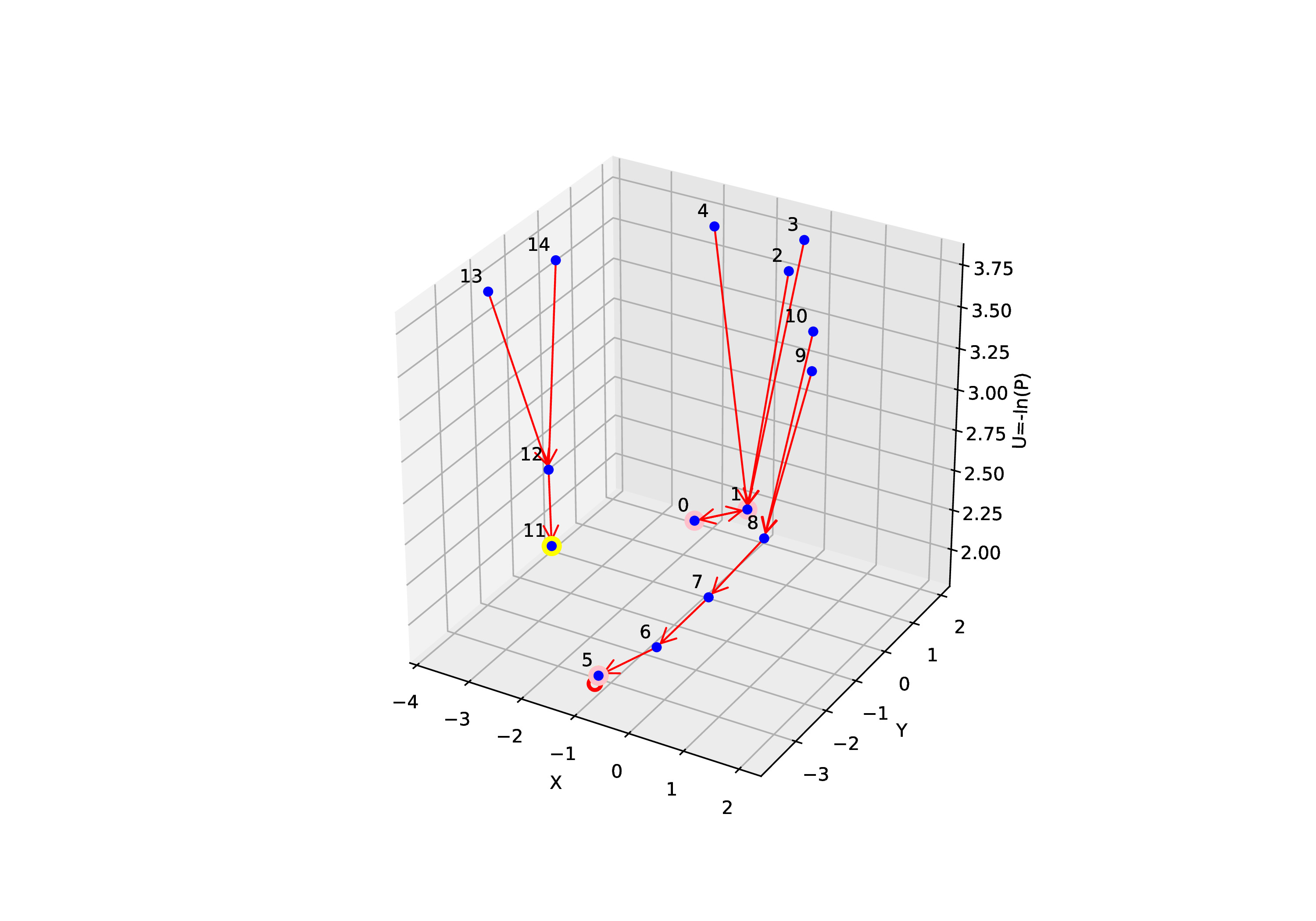
Our intuitive method [1] generated 3D view of the Boolean network attractors landscape
Below, we provide a plot of the 3D Boolean network attractors landscape for the toy model. The 3D landscape plotted is consistent with the idea proposed by Waddington's epigenetic landscape where attractors are located at the bottom of the landscape for representing cell states.
 Based on the state transition graph above we know node 11 is point attractor. Whereas node 0 and node 1 forms a cyclic attractor. Node 5 has a self loop and can be classified as
cyclic attractor as well.
References
1. Chong, K. H. An intuitive method to visualize Boolean network attractors landscape based on probability distribution from trajectories. bioRxiv 2024–10(2024).
2. Zhang, X., Chong, K. H., Zhu, L. & Zheng, J. A Monte Carlo method for in silico modeling and visualization of waddington’s epigenetic landscape with intermediate details. Biosystems 198, 104275 (2020).